Water Exchange Market

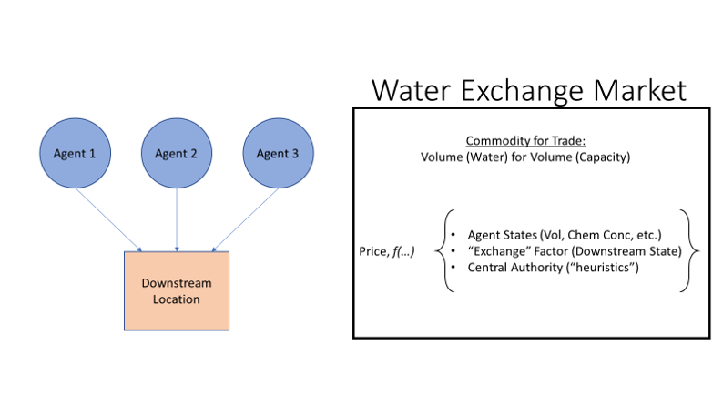
Agents are upstream locations that have a control volume and control point associated with it. For every agent, \(i\), we can define their wealth, \(W_i\), as a function of their normalized characteristic states. In the simplest case of the single characteristic of volume, wealth can be defined as:

\(W_i = \mu_i \times V_i\)

Where:

• \(\mu_i\) is a weighting parameter, and
• \(V_i\) is the volume within the control volume, normalized to the maximum volume possible within the control volume.

Wealth of any agent can be calculated using a variety of different characteristics in a variety of forms. We haven’t (yet) experimented with wealth formulations which are not linear, but we could explore it. Practical limitation to the number of agent characteristics included in the Wealth calculation is the total number of characteristics measured in your system at all agent locations.

The price of the traded commodity (in this case Volume), \(P_V\), in an exchange is:

\(P_V = \frac{\sum_{i=1}^{n} W_i + EF}{n + 1}\)

Where:

• \(\sum_{i=1}^{n} W_i\) is the sum of wealth of all the agents active in the Exchange,
• \(n\) is the total number of agents active in the exchange, and
• \(EF\) is the Exchange Factor. (In previous versions, this is the downstream term.)

\(EF\) should account for market conditions not associated with agent characteristics. These could include conditions at the downstream, WRRF, or outfalls. One way to define \(EF\) is

\(EF = (V_{down} - setpt) \times \beta\)

Where:

• \(V_{down}\) is the measured normalized volume at the downstream
• \(setpt\) is the operator-defined setpoint (normalized) for the downstream, and
• \(\beta\) is a weighting parameter for the downstream.

After the commodity price, \(P_V\), has been determined by the market function, Purchasing Power for each agent, \(Power_i\), is calculated as follows:

\(Power_i = max ( W_i - P_V , 0 )\)

Available supply on the exchange, \(S\), is calculated as:

\(S = ( 1 - V_{down} ) \times V_{max}\)

Where:

• \(V_{down}\) is the measured normalized volume at the downstream
• \(V_{max}\) is the maximum volume at the downstream

Knowing the Exchange’s supply and each agent’s purchasing power, we can calculate quantity of the commodity (volume) to be traded for an agent, \(V_{traded,i}\) as:

\(V_{traded,i} = S \times Power_i\)

With \(V_{traded,i}\) in hand, each agent can determine the physical/hydraulic action required to release this amount of volume to the downstream.