Building SVG Dashboard Graphics ¶

Here we will cover the scripts that builds the real-time graphic used as part of the grafana dashboard (seen below.)

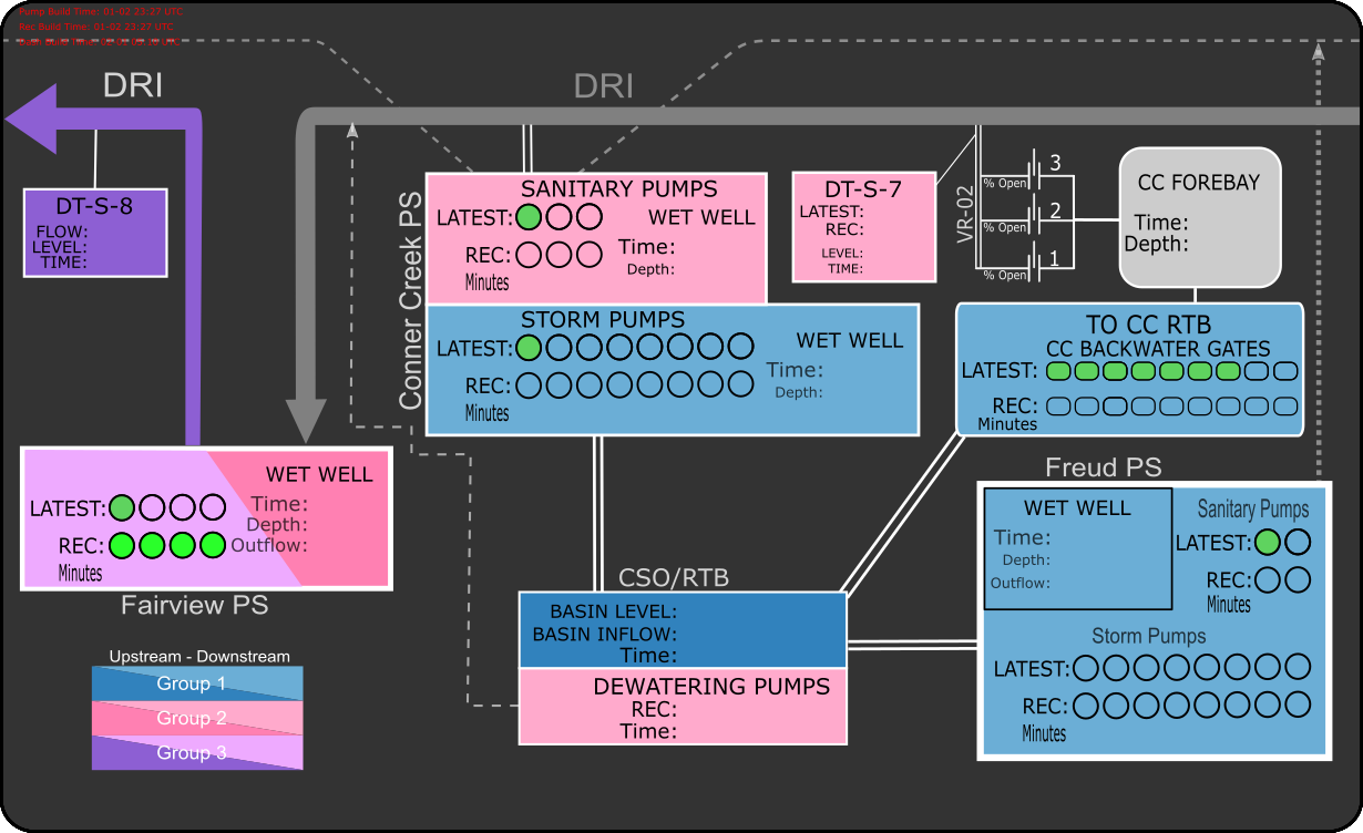
Example output of the scripts.

Scripts Called ¶

Together, three scripts and a command line operation in command_queue.py build the real-time graphic. These calls are:

python latest.py
python recommended.py
python build_full_svg.py
inkscape --export-png=/out/path/here.png /input/path/here.svg

Graphics File Structure ¶

First, however, it is worthwhile to discuss the directory and file structure that these scripts leverage to build the graphics.

Essentially, what these scripts do is select object layers within pre-built .svg files and stack those layers on top of the default base layer. Once these layers are collected into a single file, it is then exported as a .png file for upload to the cloud.

Navigating from the root directory of the repo, the file structure for the graphics is: .\GRAPHICS\{Pumpstation Name}\{Current Or Recommendation}\{Wet Well}\{# of Pumps}.svg

Where:

{Pumpstation Name} is the same name used for the measurement name during the database query (ex. FAIRVIEW)
{Current Or Rec} refers to whether the path is for a real or recommended state
{Wet Well} refers to the location within the pump station, as many of the stations have both a sanitary (SN) and storm (ST) wet wells. (CONNER folder has an additional term for the sewer gates (SG) because that gates are associated with the measure.)
{# of Pumps}.svg is the file which corresponds to a given number of pumps ON for a wet well, either recommended or real, for a pumpstation.

For example, if the control engine were recommending Conner Creek Pump Station have five, 5, of its storm pumps ON, then the file to include in the build of the dashboard for this information would be:

.\GRAPHICS\CONNER\REC\ST\5.svg

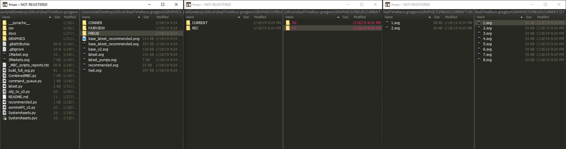
Example file structure of GRAPHICSdirectory.

latest.py ¶

latest.py first establishes a connection with the InfluxDB instance and processess the database field(s) to query.

Next, we instantiate our pumpstation objects.

Using the method .query_measures(), pump and gate measurements are queried from the database. The .pumps_running() method counts and stores the number of pumps for each station that have the status ON. Likewise, the .gates_open() accomplishes the same task, but for gates. With the number of pumps and gates of status ON known, the corresponding .svg filenames for each pumpstation is collected in the list add_to_base. This all is accomplished in the for loop below.

Next, using the module svgutils, the .svg are loaded into an object layer and is appended into a list. The contents of the list are combined and saved to the file latest.svg. The result is a file with green objects that correspond to the number of pumps or gates ON at pumpstations across the network. An example is below.

Sample output of latest.py

recommended.py ¶

recommended.py performs the same procedure as latest.py. The difference is instead of building an .svg file corresponding to the latest states in the system it builds an .svg file corresponding to the most recent recommended states as determined by the control calculations in Market-Based Control Recommendation Engine. An example is below.

Sample output of recommended.py

build_full_svg.py ¶

build_full_svg.py takes the objects located in latest.svg and recommended.svg and adds them to the base layer in base_v2.svg. The result can be seen in the figure below.

Completed output of scripts.

Inkscape Command Line ¶

Finally,

inkscape --export-png=/PATH/TO/GRAPHICS/base_latest_recommended.png /PATH/TO/GRAPHICS/base_latest_recommended.svg

converts the .svg output into a .png file. Learn more about Inkscape here.